Polarion
Polarion ALM 2404 – What’s New and Noteworthy
April 24, 2024
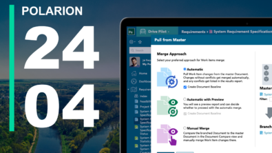
Polarion ALM 2404 brings new automatic merge, test management improvements, new security features, extended REST APIs, and numerous user experience improvements. Learn more in our blog!